The TMS Electric Field

This being my first post to this newly established blog I wish to start from the fundamentals. And, as I see it, I great place to start is the description of the magnetic field ${\bf B}({\bf r},t)$ and the electric field ${\bf E}({\bf r},t)$ that can be established within biological tissue due to an external current source. In transcranial magnetic stimulation (TMS) experimentation the biological tissue is usually a mammalian head. To a good approximation (good enough to understand many important features TMS fields) we may model the head as a homogeneous spherical conductor of volume $V$ , conductivity $\sigma_s$ , magnetic permeability $\mu_s$ and permittivity $\epsilon_s$ . In TMS a current density, that is supported external to $V$ only, provides the source of the electromagnetic fields within the spherical conductor.

I will rely on vector spherical harmonics in the derivation given below. This a natural choice given the symmetry of the idealized spherical conductor model. An excellent treatment of vector spherical harmonics is given by Varshalovich et al [5]. Most of the earlier treatment of the electric field within a spherically symmetric conductor did not make use of vector spherical harmonics and as a result the derivations were long and cumbersome [1]. I know of only one paper [8] or text making use of vector spherical harmonics in the treatment of this physical problem. This blog post will fill in details that were absent or glossed-over within that publication and hopefully make it easier for the reader to understand the derivation as well as the various physical assumptions that come into mathematical play.

I. Preliminaries

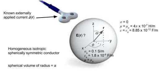
Figure 1 depicts the spherical conductor model that will be used. The figure lists appropriate estimates [6] of the conductivity, permittivity and permeability within the spherically symmetric conductor of radius $a$ and external to it. We will assume that prior to turning on the external applied current ${\bf J}({\bf r},t)$ the charge density $\rho ({\bf r},t)$ is everywhere zero.

TMS Study Group 3_ Physics of the E field in spherical conductor — Fig 1: Assumed physical parameters for the spherical conductor model

We want to determine ${\bf E}({\bf r}, t)$ within the conducting sphere. Since for time varying electromagnetic fields ${\bf E}({\bf r}, t)$ is given by

${\bf E}({\bf r},t) = - \nabla \Phi({\bf r}, t) - \frac{1}{c} \frac{\partial{\bf A}({\bf r}, t)} {\partial t} \qquad \qquad \qquad \qquad \qquad \qquad \qquad \qquad (1)$

we will need to determine the scalar potential $\Phi({\bf r}, t)$ and magnetic vector potential ${\bf A}({\bf r}, t)$ . Before taking on that task we cover a few physical and mathematical preliminaries.

Surface Charge Density

To determine the scalar potential $\Phi({\bf r}, t)$ we will need to understand an important feature of the charge density for homogeneous media where the only source of current is Ohmic currents: The charge density is zero everywhere within the conductor but possibly nonzero at its surface. We can see this as follows. According to Maxwell-Ampere Law we can write

$\nabla \times {\bf B}({\bf r},t) = \frac{1}{c} \frac{\partial{\bf E}({\bf r}, t)} {\partial t} + \frac{4\pi}{c} {\bf J}({\bf r}, t). \qquad \qquad \qquad \qquad \qquad \qquad \qquad \quad (2)$

And when the total current ${\bf J}({\bf r}, t)$ is due only to ohmic current such that ${\bf J}({\bf r}, t) = \sigma {\bf E}({\bf r}, t)$ then

$\nabla \times {\bf B}({\bf r},t) = \frac{1}{c} \frac{\partial{\bf E}({\bf r}, t)} {\partial t} + \frac{4\pi}{c} \sigma {\bf E}({\bf r}, t).$

It’s helpful to Fourier transform the above equation to the following frequency-space equivalent

$\nabla \times {\widetilde{\bf B}}({\bf r},\omega) = \frac{i\omega}{c} {\widetilde{\bf E}}({\bf r}, \omega) + \frac{4\pi}{c} \sigma {\widetilde{\bf E}}({\bf r}, \omega)$

where the tilde denotes a Fourier transformed quantity. If we take the divergence of both sides of this equation to get

$0 = i\omega \nabla \cdot {\widetilde{\bf E}}({\bf r}, \omega) + 4\pi \nabla \sigma \cdot {\widetilde{\bf E}}({\bf r}, \omega) + \sigma \nabla \cdot {\widetilde{\bf E}}({\bf r}, \omega)$

and then use the Maxwell Law $\nabla \cdot {\widetilde{\bf E}}({\bf r},\omega) = 4\pi {\widetilde \rho}({\bf r},\omega)$ we find

${\widetilde \rho}({\bf r},\omega) = - \frac{1}{\sigma + i \omega} \nabla \sigma \cdot {\widetilde{\bf E}}({\bf r}, \omega).$

Within a uniform conductor $\nabla \sigma = 0$ and therefore the charge density within the conductor is zero according to the above equation. At the surface, on the other hand, $\nabla \sigma \ne 0$ therefore a nonzero surface charge density may be present. This of course applies in temporal-space as well as frequency-space. Note that if we had used a spherically symmetric model with multiple spherically symmetric conductivity boundaries (rather than just one at the surface of the sphere) then there would be multiple spherical layers of surface charge, one at each boundary.

Ohmic Current Contribution to the Vector Potential

The applied external current (TMS coil current) will produce a time-varying magnetic field within the conductor and hence an electromotive force. The electromotive force will in turn induce ohmic current in the spherically symmetric conductor. However these internal currents can be neglected when calculating the vector potential ${\bf A}({\bf r}, t)$ in biological media. This argument can be made by considering the skin-depth for this spherical conductor at the usual TMS frequencies (or smaller).

The induced ohmic current within the spherical conductor must oppose the time varying magnetic field which created it according to Lenz’s Law and this opposition is responsible for the decay of field strength with distance from the surface of the conductor. The characteristic length for this decay is known as the skin depth and is a measure of how significant the induced ohmic currents are in their contribution to the total magnetic field. If the skin depth for the spherical conductor is large compared to the size of the sphere then it is safe to assume that the ohmic currents within the spherical conductor contribute little to the magnetic field as compared to the externally applied current which produced them.

The skin depth $\delta$ for an arbitrary conductor is given by [6]

$\delta = (2\pi f)^{-1} \sqrt{[\sqrt{1+(\sigma/2\pi f \epsilon)^2} - 1 ]\mu \epsilon/2 }$

Using the assumed constants the skin depth is 0.8 m at f = 10 kHz which is of course much larger than the size of a human head. We may therefore neglect the contribution to the vector potential due to the internal ohmic current.

To elaborate a bit further consider that TMS experiments (using coils with 4000 A current magnitude) are known to generate internal ${\bf E}({\bf r}, t)$ fields of magnitude 100 V/m near the surface of the brain. Since the conductivity of biological tissue is approximately 0.1 S/m then a reasonable estimate for the current density of the ohmic internal currents would be 10 A/m². The current within the TMS coil is usually more than 1000A and flows through a conductor with a cross sectional area of approximately 0.00003 m². This gives a current density of more than 33,000A/m². Clearly with the TMS coil placed near the surface of the sphere the contribution to the vector potential due to the externally applied current easily dominates that due to the internal ohmic current.

The existence of the internal current is, however, important in that it gives rise to surface charge density mentioned previously and its associated scalar potential $\Phi ({\bf r}, t)$ . One may from the outset have a good reason to suspect that the surface charge plays a non-negligible role in the character of the electric field but that is something that we will verify as we continue with the calculation of the electric field ${\bf E}({\bf r}, t)$ .

Negligible Polarization and Magnetization Current

Also within the spherical conductor we note that the other two possible contributions to electric current within linear media, the polarization current and the magnetization current, are too small to be of consequence. The polarization current $\frac{\partial \bf P}{\partial t} = \epsilon_s \frac{\partial \bf E}{\partial t}$ for a sinusoidal varying E field of frequency 4 kHz and amplitude 100 V/m would be (using $\epsilon_s$ supplied in Figure 1) approximately 0.0045 A/m² a value which is orders of magnitude smaller than that due to ohmic current. Also since the magnetic permeability of the sphere is taken to be approximately equal to that of the vacuum we can expect the magnetization current to be negligible as well.

The Boundary Condition: Linking the External Current and the Surface Charge

Lastly we establish the boundary condition on the electric field at the surface of the spherically symmetric conductor. This boundary condition will allow us to determine the a priori unknown surface charge density (or a particular representation of it) in terms of the externally applied current.

Since the wavelength associated with frequencies employed in TMS work (usually no greater than 10 kHz) are very large compared with the size a human head (and hence our spherically symmetric conductor) we will be able to use the typical quasistatic form of the vector potential and scalar potential in which propagation effects can safely be neglected. The quasistatic approximation amounts to a neglect of the first term on the right side of Equation (2) and if one takes the divergence of that equation one finds that $\nabla \cdot {\bf J}({\bf r}, t) = 0$ everywhere. By constructing an infinitesimal Gaussian pillbox at the surface of the conductor and using the fact that there is no current external to the conductor then the condition $\nabla \cdot {\bf J}({\bf r}, t) = 0$ yields ${\hat {\bf r}} \cdot {\bf J}({\bf r}, t) = 0$ at $r =a$ . And since ohmic currents are the only significant currents within the conductor we may write the boundary condition as ${\hat {\bf r}} \cdot {\bf E}({\bf r}, t) = 0$ at $r =a$ . That is, the component of the electric field normal to the surface of the spherical conductor is zero at the surface.

II. Determining the Vector and Scalar Potentials

The quasistatic form of the vector potential and scalar potential is identical to that for static fields albeit with time dependent charge and current densities. We now write a convenient form for the vector and scalar potentials which makes use of vector spherical harmonics and scalar spherical harmonics respectively. To the resulting equations we will later apply the boundary condition to determine some unknown coefficients related to the surface charge density.

The Vector Potential

The vector potential in the quasistatic case is given by

${\bf A}({\bf r},t) = \frac{1}{c} \iiint \frac{{\bf J}({\bf r}',t)}{|{\bf r} - {\bf r}'|} d^3{\bf r}'.$

Expanding the integrand in terms of vector spherical harmonics (see [5] pg 229) we can write

${\bf A}({\bf r},t) = \frac{4 \pi}{c} \sum\limits_{ljm} \frac{r^l}{2l+1} {\bf Y}^l_{jm}(\theta,\phi) \iiint \frac{1}{r'^{l+1}} {\bf J}({\bf r}',t) \cdot {\bf Y}^{*l}_{jm}(\theta',\phi') r'^2 \sin \theta' dr' d\theta' d\phi'$

which can be compactly written as

${\bf A}({\bf r},t) = \sum\limits_{ljm} \frac{r^l}{2l+1} {\bf Y}^l_{jm}(\theta,\phi) A^l_{jm}(t)$

where

$A^l_{jm}(t) = \frac{4 \pi}{c} \iiint \frac{1}{r'^{l+1}} {\bf J}({\bf r}',t) \cdot {\bf Y}^{*l}_{jm}(\theta',\phi') r'^2 \sin \theta' dr' d\theta' d\phi'.$

Since the applied current is assumed to be known then the coefficients given above are known as well. The equation for the vector potential given above applies to any current density. However the current of our spherically symmetric conductor is more restrictive. As noted previously, according to the quasistatic approximation we may write $\nabla \times {\bf B} = {\bf J}$ (Recall that this implies that $\nabla \cdot {\bf J} = 0$ .). Since, as noted in the preliminaries, the internal ohmic current can be neglected in the calculation of the vector potential then it follows that within the spherical conductor we may write $\nabla \times {\bf B} = \nabla \times \nabla \times {\bf A} = 0$ . Applying this constraint (making use of identities given in [5] pg 217) one finds that $A^{j+1}_{jm}(t) = 0$ and therefore

${\bf A}({\bf r},t) = \sum\limits_{jm} \left[ \frac{r^j}{2j+1} {\bf Y}^j_{jm}(\theta,\phi) A^j_{jm}(t) + \frac{r^{j-1}}{2j-1} {\bf Y}^{j-1}_{jm}(\theta,\phi) A^{j-1}_{jm}(t) \right]. \qquad \qquad \qquad \qquad (3)$

For the sake of completeness we also write the corresponding expression for the magnetic field ${\bf B} = \nabla \times {\bf A}$ within the spherically symmetric conductor

${\bf B}({\bf r},t) = i \sum\limits_{jm} \sqrt{\frac{j+1}{2j+1}} r^{j-1} {\bf Y}^{j-1}_{jm}(\theta,\phi) A^j_{jm}(t) .$

The Scalar Potential

The scalar potential in the quasistatic approximation is given by

$\Phi({\bf r},t) = \iiint \frac{\rho({\bf r}',t)}{|{\bf r} - {\bf r}'|} d^3{\bf r}'$

Proceeding in a manner similar to that for the vector potential we apply the spherical harmonic expansion of $1/{|{\bf r} - {\bf r}'|}$ applicable to the interior of the sphere (see [5] pg 165-166) to obtain

$\Phi({\bf r},t) = 4\pi \iiint \rho( r', \theta', \phi', t) \sum\limits_{jm} \frac{1}{2j+1} \frac{r^j}{r'^{j+1}} Y_{jm}(\theta,\phi) Y^*_{jm}(\theta',\phi') r'^2 \sin \theta' dr' d\theta' d\phi'$

Since the charge is distributed on the surface of the sphere only we write the surface charge density as

$\rho(r, \theta, \phi, t) = \frac{1}{4\pi r^2} \delta(r-a) \rho_s(\theta,\phi,t)$

where $\rho_s(\theta,\phi,t)$ gives the angular dependence of the surface charge density. Integrating with respect to $r'$ we obtain

$\Phi({\bf r},t) = 4\pi \iint \rho_s( \theta', \phi', t) \sum\limits_{jm} \frac{1}{2j+1} \frac{r^j}{a^{j+1}} Y_{jm}(\theta,\phi) Y^*_{jm}(\theta',\phi') \sin \theta' d\theta' d\phi'$

which can be written compactly as

$\Phi({\bf r},t) = \sum\limits_{jm} \frac{r^j}{2j+1} Y_{jm}(\theta,\phi) C_{jm} (t)$

where

$C_{jm}(t) = \frac{1}{a^{j+1}} \iint \rho_s( \theta', \phi', t) Y^*_{jm}(\theta',\phi') \sin \theta' d\theta' d\phi'.$

III. Determining the Electric Field

Our task is to find the a priori unknown $C_{jm}(t)$ in terms of the known $A^l_{jm}(t)$ . We do this by applying our previously established boundary condition for the component of $\bf E$ normal to the surface (the radial component) at $r=a$ . Recall that our boundary condition is

$0 = [{\bf E}({\bf r}, t) \cdot {\hat {\bf r}}]_{r=a} = \left[ \nabla \Phi({\bf r},t) \cdot {\hat {\bf r}} + \frac{1}{c} \frac{\partial{\bf A}({\bf r}, t)}{\partial t} \cdot {\hat {\bf r}} \right]_{r=a}$

To apply the boundary condition first we calculate $\bf E$ inside the sphere by substituting our results for the scalar and vector potentials into Equation (1) to obtain

${\bf E}({\bf r}, t) = \sum\limits_{jm} C_{jm}(t) \sqrt{\frac{j}{2j+1}} r^{j-1} {\bf Y}^{j-1}_{jm}(\theta,\phi) \\ \indent \indent \indent \!\! + \frac{1}{c} \sum\limits_{jm} \left[ \frac{\partial A^j_{jm}}{\partial t} \frac{r^j}{2j+1} {\bf Y}^j_{jm}(\theta,\phi) + \frac{\partial A^{j-1}_{jm}}{\partial t} \frac{r^{j-1}}{2j-1} {\bf Y}^{j-1}_{jm}(\theta,\phi)\right]. \qquad \quad \; (4)$

The normal component of the electric field evaluated at the surface of the sphere is then given by (see [5] pg 219 for applicable identities)

$[{\bf E}({\bf r}, t) \cdot {\hat {\bf r}}]_{r=a} = \sum\limits_{jm} \left[ \frac{j}{2j+1} C_{jm}(t) + \frac{1}{c} \frac{1}{2j-1} \frac{j}{2j+1} \frac{\partial A^{j-1}_{jm}}{\partial t}\right] a^{j-1} Y_{jm}(\theta,\phi).$

Equating the above equation to zero the boundary condition then yields

$C_{jm}(t) = - \frac{1}{c(2j-1)} \sqrt{\frac{2j+1}{j}} \frac{\partial A^{j-1}_{jm}}{\partial t}. \qquad \qquad \qquad \qquad \qquad \qquad \qquad \qquad (5)$

Finally we substitute Equation (5) into Equation (4) to obtain the electric field $\bf E$ inside the sphere:

${\bf E}({\bf r}, t) = \frac{1}{c} \sum\limits_{jm} \frac{\partial A^j_{jm}}{\partial t} \frac{r^j}{2j+1} {\bf Y}^j_{jm}(\theta,\phi) \qquad \qquad (6)$

IV. Wrapping Things Up: Important TMS Electric Field Features

Equation (6) allows us to make the following important statements about the electric field established by a TMS coil.

(1) First we note that the vector spherical harmonic appearing in the above expression is given by (see [5] pg 210-211):

${\bf Y}^j_{jm}(\theta,\phi) = -{\bf e}_{\theta} \frac{m}{\sqrt{j(j+1)}} \frac{1}{\sin \theta} Y_{jm} (\theta,\phi) -{\bf e}_{\phi} \frac{i}{\sqrt{j(j+1)}} \frac{\partial Y_{jm} (\theta,\phi)}{\partial \theta}$

which has no radial component. Therefore the electric field within the spherically symmetric conductor is always tangential to the surface of the sphere. Since this was established for an arbitrary current density this means that no TMS coil geometry or orientation of that coil relative to a head can ever establish a radial component to the electric field. This holds so long as the spherically symmetric conductor model is a reasonable model for the head.

(2) We have little control over the radial dependence of the field. It always falls off as one approaches the origin of the sphere and the fall off increases with the index $j$ . As a consequence, since the vector spherical harmonics of larger index $j$ contain more spatial detail, if the E field appears rather focal on a spherical shell of radius $r$ it will be less focal as $r$ decreases. Also there can be no selective E field targeting of brain tissue at depth within the head.

(3) We have some control over the angular distribution of the tangentially oriented E field but at any point $r$ it is limited to the subspace of the ${\bf Y}^j_{jm}(\theta,\phi)$ vector spherical harmonics. This is topic that needs further exploration. What types of E fields with focal angular distribution are possible?

(4) The electric field depends upon the temporal derivative of the coefficients describing the externally applied current.

References

[1] H. Eaton: Electric Field Induced in a Spherical Volume Conductor from Arbitrary Coils: Application to Magnetic Stimulation and MEG, Medical and Biological Engineering and Computing, Vol. 30, No. 4, July 1992, pp. 433 – 440.

[2] M. Bencsik, R. Bowtell and R. M. Bowley: Electric fields induced in a spherical volume conductor by temporally varying magnetic field gradients, Phys. Med. Biol., Vol 47, 2002, 557-576.

[3] K. Porzig, H. Brauer, Hannes Toepfer: The Electric Field Induced by Transcranial Magnetic Stimulation: A Comparison Between Analytic and FEM Solutions, Serbian Journal of Electrical Engineering, Vol. 11, No. 3, 2014, 403-418.

[4] R. Plonsey and D. B. Heppner: Considerations of Quasi-stationarity in Electrophysiological Systems, Bulletin of Mathematical Biophysics,, Vol 29, 1967, 657-664.

[5] D. A. Varshalovich, A. N. Moskalev and V. K. Khersonskii, Quantum Theory of Angular Momentum, World Scientific, 1988, 208-229.

[6] J. P. Reilly, Electrical Stimulation and Electropathology, Cambridge University Press, 1992, pg 22.

[7] J. D. Jackson, Classical Electrodynamics, 2nd edition, pg 391-394.

[8] L. M. Koponen, J. O. Nieminen, R. J. Ilmoniemi, Minimum-energy Coils for Transcranial Magnetic Stimulation: Application to Focal Stimulation, Vol 8, 2015, 124–134.

PractiCalTMS

Discussing Transcranial Magnetic Stimulation